Managing the Processing Parameters
Algorithm
The core of Delph INS Subsea is based on the unscented Kalman filter algorithm implemented in the INS. This filter provides an optimal integration of inertial and external data. The computation process is based on models of aiding sensors and inertial sensors errors. The error models of aiding sensors are specific for each type of aiding sensor.
Two types of algorithms are used:
| > | Basic Algorithm: uses the same principle as in real-time processing |
| > | Optimized Algorithm: post-processing is done in three phases. |
| ● | Forward computation from the beginning to the end of the survey |
| ● | Backward computation which reverses time and processes data backwards from the end to the beginning of the survey |
| ● | Merging of both forward and backward computations to get an accurate and smooth result. |
You can choose the Basic Algorithm to adjust parameters and move to Optimized Algorithm to achieve the best performance since it is three times longer than the basic algorithm.

|
When processing data in Optimized mode please check the following:
|
|||||||||
Principle of Optimized Processing
The basic inertial processing algorithm consists in the integration of time series of data (gyrometers, accelerometers, aiding sensors) chronologically. This algorithm can reverse, it means that time series are reversed and data are integrated from the end to the beginning. After processing a data set in both « directions » the two results can be merged.
During the first stage of processing (the forward pass) data are integrated chronologically. The Kalman filtering operation is a recursive operation, each calculated point is the result of treatment of all previous points, the estimates become more precise as one gets closer to the end of the file.
During the second stage of processing (the backward pass) data are integrated anti-chronologically from end of file to beginning. Each calculated point is the result of treatment of all points that follow, the estimates become more precise as one gets closer to the beginning of the file.
During the last stage of processing (the smoothing pass) the two previous results are merged, each calculated point is the result of processing all points on the line, the estimates precision is therefore optimal for the whole file.
The following figure shows the error of position of the INS during an aiding sensor outage; it means the INS runs in free inertial mode during this section:
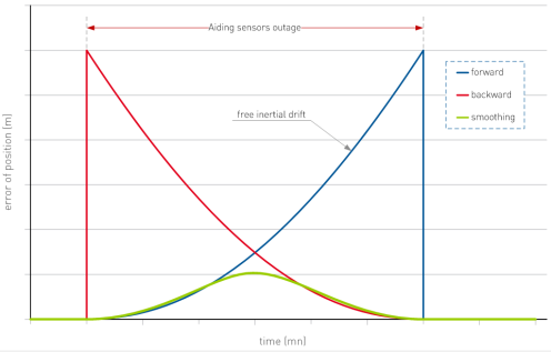
Error of position with forward, backward and both algorithms
The blue curve is the error of position during the forward pass. It increases in a parabolic manner during the aiding sensor outage.
The red curve is the error of position during the backward pass. It is the symmetrical of the forward result. The fusion of the results produces the green curve that takes the best of each.
Procedure
| 1. | In the Processing panel, expand the INS processing parameters. |
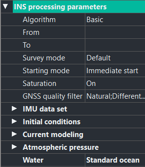
| 2. | Click on the right of Algorithm and select the type (Basic or Optimized). |
| 3. | Enter the From and To values (optional) to define the beginning/end interval in which you want to apply the processing. By default, all data is processed from the start to the end. The two fields enable decreasing the processed period. During the first minutes following the beginning of the processing, the trajectory must meet the alignment constraints encountered in real time with the INS (coarse alignment, fine alignment) (refer to the INS user manuals). |
Choosing the start of the processing on a non-adequate period considerably decreases the performance and this cannot be measured.
Note: Be careful if you change the beginning time to choose a static period.
| 4. | Set the Survey Mode field to Default. |
In the case where the INS is not used in a standard way, it is possible to modify this value. Set the Survey Mode to Hydro, in the case, for example, where INS is used on a surface vessel in order to achieve a hydrographic survey, This choice has the effect to apply specific parameters during the processing.
| 5. | Click on the right of Starting mode and choose the mode: Immediate run, Wait for position or Wait for speed. |
| 6. | Click on the right of Saturation and choose to take the saturation into account or not. |
In real time, the inertial products have saturation thresholds depending on the environment (subsea, land, air). When the system is in saturation, all data is frozen.
It is recommenced to set the saturation to 'Yes' to have a behavior similar to the real time.
The saturation can be set to 'No' for exceptional replay situation (high speed aircraft)
| 7. | Click on the right of GNSS quality filter in order to filter the data by ticking one or several types of GNSS: |
| > | Natural |
| > | Differential |
| > | PPS |
| > | RTK fixed |
| > | RTK float |
By default, if no filtering was done in real time, all GNSS quality values are ticked and used.
If one box is unticked, the corresponding GNSS mode is pre-filtered: any measure coming with this mode is ignored by the Kalman filter.
| 8. | Expand IMU data set: the begin time, end time and survey duration are displayed (not editable). |
| 9. | Expand Initial conditions, select in the pull-down menu the position mode: |
| > | Automatic (recommended): retrieves the first GPS |
| > | User defined: is by default the “initial position” stored in the INS, which can be meaningless. You can edit the values. |
It is very important to enter an accurate initial position, as even an error of a few hundreds of meters can degrade in the post-processing performance.
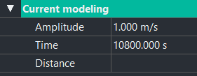
| 10. | Expand Current Modeling, enter an Amplitude, a Time and a Distance. If you let these fields empty the default values are amplitude: 0.5 m/s, time: 3 h, distance: 20 km. |
| 11. | Expand Atmospheric pressure, you may let the Default Value empty (in this case the default value is 1013.25 hPa) or drag and drop a atmospheric pressure data file from the Variables panel to Data File and Channel. |
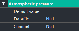
If the pressure sensor used delivers a pressure relative to the surface, enter 0.0 in the Atmospheric pressure / Default value field, so that atmospheric pressure is not subtracted twice.
The atmospheric pressure data are used to convert the pressure measurements in immersion described in Adding a Water Profile.
| 12. | Expand Water. You may choose between Standard ocean, Average density and Density profile. For more information, see Adding a Water Profile. |